Signalverarbeitung mit MATLAB und Künstlicher Intelligenz

Abb. 1: Signalverarbeitung mit MATLAB^® und Künstlicher Intelligenz

Autor:	Moye Nyuysoni Glein Perry
Art:	Project Work
Starttermin:	14.11.2024
Abgabetermin:	31.03.2025
Betreuer:	Prof. Dr.-Ing. Schneider

Abstract

In modern engineering, signal processing forms a fundamental basis for analyzing and enhancing data from various sources. With the coming of artificial intelligence (AI), traditional signal processing techniques can be even replaced by AI methods capable of addressing increasingly complex tasks. This article presents an integrative project that applies MATLAB as the core platform for signal processing while incorporating AI techniques. The work includes a comprehensive study of image processing tasks, such as object detection and classification, and provides a comparative evaluation between classical algorithms and AI-based approaches. The methodology is rigorously documented through scientific research, systematic experimentation, and the use of visual aids like mind maps and annotated results.

Fig. 2: Project MindMap

Introduction

Signal processing has long been a basis in the analysis and manipulation of data in various domains such as telecommunications, radar, audio processing, and imaging. Signal processing has traditionally focused on analyzing, filtering, and interpreting signals in both the time and frequency domains. With the integration of AI, especially deep learning, the possibilities expand to include noise reduction and more. It is essential in many modern applications such as communications, audio and image processing, biomedical signal analysis, and control systems.

MATLAB’s extensive toolboxes for both digital signal processing (DSP) and machine learning allow for the exploration of new approaches that can potentially offer improved performance and robustness in handling noisy or complex signals.

Time planning/project plan

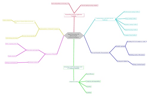
The project schedule was represented using Gantt charts. Figure 3 and 4 shows the original plan. Everything I planned on working on was showned as well on my mind map in Fig. 2

Signal Processing Fundamentals

Time Domain vs. Frequency Domain

Time Domain: Time-domain analysis involves studying a signal as it varies over time. However, it might be challenging to extract features such as periodicity or noise characteristics directly from the time domain.

Frequency Domain: Converting a signal into its frequency components (using techniques like the Fourier Transform) often makes it easier to identify and filter out noise, detect repeating patterns, or study signal behavior over various frequency bands.

Signals:

A signal is any piece of information that changes over time or space and can be measured. It may be continuous (analog) or discrete (digital).

Transforms:

Techniques like the Fourier Transform and the Discrete Wavelet Transform decompose signals into constituent frequency (or time-frequency) components for easier analysis.

Filtering:

The process of removing unwanted noise or extracting useful parts of a signal. Techniques include low-pass, high-pass, band-pass, and adaptive filters.

Low Pass Filters: Permit signals with frequencies lower than a cutoff frequency, useful for removing high-frequency noise.

High Pass Filters: Permit frequencies higher than a cutoff frequency, often used to eliminate low-frequency drift or interference.

Band Pass and Band Stop Filters: Focus on specific frequency bands.

cutoff frequency: The cutoff frequency, or cutoff, determines where the signal is cut off. If a signal contains frequencies that range from 500 Hz up to 8000 Hz and the cutoff frequency is set at 4000 Hz, frequencies above 4000 Hz are filtered, for example, in the case of low-pass filters.

Fig. 3: Gannt Chart

Fig. 4: Gannt Chart Continuation

Fast Fourier Transform (FFT) and Discrete Cosine Transform (DCT)

FFT: Extracting Frequency Components Purpose: The FFT is used to decompose a signal into its constituent frequency components quickly. It is particularly effective for analyzing periodic signals.

What It Does: Computes the amplitude and phase of frequency components.

DCT: Energy Compaction and Compression Purpose: The DCT transforms a signal into a sum of cosine functions oscillating at different frequencies. It is popular in image and audio compression (e.g., JPEG, MP3) due to its energy compaction properties.

What It Does: Concentrates energy into a few low-frequency coefficients, which is beneficial for compression.

Frequency Over Time: Why Shift to Frequency Analysis?

Working in the frequency domain allows for:

Filtering Unwanted Frequencies: Easily design filters to isolate or remove specific bands.

Feature Extraction: Many machine learning models perform better when provided with frequency domain features rather than raw time signals.

Noise Reduction: Identify and remove noise that might not be apparent in the time domain.

Literature Review

According to Oppenheim and Schafer (2009), classical signal processing uses statistical and deterministic techniques like Fourier transforms. Despite their strength, these techniques frequently lack flexibility and necessitate manual parameter adjustment.

On the other hand, deep learning models—particularly CNNs and YOLO networks—have proven to be more effective at interpreting signal and visual data. Transfer learning makes it possible to use previously learned information for domain-specific applications by utilizing frameworks such as ResNet or MobileNet. When used in control systems, reinforcement learning presents a viable approach to dynamic system optimization (Sutton & Barto, 2018).

MATLAB offers a platform for hybrid techniques by bridging both areas using toolboxes such as the Deep Learning Toolbox and Signal Processing Toolbox. The current research is based on this integration.

Methodology

Project Planning

• Created a mind map, Gannt Chart and project plan based on weekly goals and feedback from the supervisor.
• Documented all tasks and progress on the university Wiki and SVN.

Data Collection and Preprocessing

• Data for lane tracking and object detection collected from JetRacer and Kaggle datasets for other projects.
• Preprocessing steps included normalization, CSV-to-MAT conversion, and labeling via dedicated tools.

AI Model Training

Lane Tracking:

• Trained CNNs using both from scratch training and transfer learning (ResNet50, MobileNetV3).
• Evaluated performance using simulated driving outputs and training curves.

Object Detection:

• Applied YOLO models for object classification (person, dog, cat).
• Used Hough Transforms for circular detection.

Implementation Tools

• MATLAB toolboxes used: Deep Learning Toolbox, Signal Processing Toolbox, Image Processing Toolbox.
• Code and models were versioned using the school’s SVN repository.

Integrating AI in Signal Processing

AI Enhancements to Signal Processing

Deep learning can extract non-linear and hierarchical features that are often hard to engineer manually. When combined with traditional signal processing:

Preprocessing: Conventional filters and transforms (FFT, DCT) are used to prepare the data.

Feature Extraction: Deep neural networks can build on these features to further identify patterns, such as anomalies in medical signals or fault detection in industrial applications.

Role of Neural Network Layers in Signal Processing

Input Layer

Function:

Receives the preprocessed signal data (it may be raw data or transformed features like FFT coefficients).

Preprocessing:

Normalization and segmentation are done to ensure consistency before feeding into the neural network.

Convolutional Layers

Function:

Commonly employed in image processing, convolutional layers can also extract localized features in time-series data by sliding filters (kernels) over input data.

Signal Processing Connection: In many cases, convolutional filters can learn to mimic traditional filters (e.g., edge detectors or frequency filters).

Activation Functions

Purpose:

Introduce non-linearity into the network.

Common Functions:

ReLU: Effective in mitigating vanishing gradient problems.

Sigmoid/Tanh: Useful for certain tasks but may suffer from saturation in deep networks.

Impact on Training: Ensure that the network learns complex mappings and performs better with non-linear data representations. Pooling Layers

Function:

Downsample the feature maps. For signals, 1D pooling layers can help reduce noise and highlight significant features.

Types:

Max Pooling: Keeps the highest value in a set of features.

Average Pooling: Averages values to retain the overall trend.

Recurrent Layers

Role in Signal Processing: Designed to handle sequential data by maintaining memory across time steps. LSTM (Long Short-Term Memory) and GRU (Gated Recurrent Unit) layers capture temporal dependencies effectively.

Why They Matter: They can model long-term dependencies in signals such as speech or medical time-series data.

Fully Connected Layers

Function:

Integrate and transform features from previous layers into final predictions (classification, regression, etc.).

Mapping: Flatten the features extracted from convolutional or recurrent layers to make a decision based on all gathered information.

Deep Learning Training: Mechanisms and Optimizers

MATLAB® AI toolboxes:

 Practical AI EXamples 

Training Workflow Step 1: Initialization

Assign random weights for all neurons in the network.

Step 2: Forward Pass

Input data is processed layer by layer.

Input → Hidden Layers: Each hidden layer computes an output using its weights and activation functions.

Hidden → Output Layer: The final layer produces predictions or classifications.

Step 3: Loss Computation

A loss function (e.g., cross-entropy for classification, mean-squared error for regression) measures the difference between predicted outputs and ground truth.

Backpropagation and Weight Update

Backpropagation: This algorithm calculates the gradient of the loss function with respect to each weight using the chain rule. In essence, it propagates the error backward from the output to the input layers.

Weight Updates: Using the gradients, weights are adjusted with learning rate and momentum considerations.

SGDM (Stochastic Gradient Descent with Momentum): Improves standard gradient descent by accelerating convergence in the relevant direction and damping oscillations.

Adam (Adaptive Moment Estimation): Combines momentum with an adaptive learning rate for faster convergence, especially useful with large datasets or sparse gradients.

Training Dynamics: Epochs and Batches Epoch: A single pass through the entire training dataset.

Batch Propagation:

Mini-Batch Gradient Descent: The dataset is divided into mini-batches (smaller subsets) so that weight updates occur more frequently than one update per epoch. This balances efficient computation with stability.

Per Epoch Calculation: With each epoch, the network processes all the mini-batches, updates weights, and reduces the overall error. Monitoring loss and validation accuracy per epoch allows you to gauge training progress and adjust hyperparameters when needed.

Function Effects:

Activation Functions (e.g., ReLU, Sigmoid): Govern how signals pass through layers, affecting non-linearity.

Optimizers (e.g., Adam, SGDM): Direct the way weight adjustments are carried out based on gradient information.

Learning Rate: A critical hyperparameter that scales the magnitude of weight updates. Too high may cause overshooting, while too low may slow convergence.

Inside the Hidden Layers Weights and Biases: Each neuron has weights (that multiply inputs) and biases (offsets) that are adjusted during training.

Activation Functions: Determine whether neurons fire (pass their input) or not, adding non-linearity.

Before Weight Changes: The network computes the loss which quantifies the error between actual output and predicted output. This loss is then used to compute gradients through backpropagation.

Backpropagation: Gradients are calculated layer by layer from the output back to the input. The optimizer then uses these gradients to update weights.

Epoch-wise Evolution: Each epoch represents a complete cycle over the training dataset. With each epoch, the loss should ideally decrease as the network learns.

Optimizers and Their Role

SGDM: Uses momentum to smooth out updates and helps in converging faster by accounting for past gradients.

Adam: Adapts the learning rate for each parameter individually by considering both the first and second moments of the gradient, which often results in faster convergence and improved performance in noisy datasets.

Image Processing

Image processing refers to the use of algorithms and computational techniques to analyse, enhance, and manipulate images. It involves altering or improving images using various methods and tools. The main aim of image processing is to improve image quality. Whether it’s enhancing contrast, adjusting colours, or smoothing edges, the focus is on making the image more visually appealing or suitable for further use. It’s about transforming the raw image into a refined version of itself.

Sample Task: Object Detection Identify in an Image

• Classical Method: Circular Objects Detection

• results:

• AI based method: Detect people, cats and dogs in message using YOLO model.

• Results

Results

Lane Tracking: CNN models successfully simulated lane following behavior with moderate accuracy. Initial data had limitations (e.g., curve bias), requiring additional data and normalization.

Object Detection: YOLO models identified multiple objects with high accuracy after fine-tuning and proper data labeling.

Signal Processing Enhancements: Classical techniques (e.g., Hough Transforms) were used alongside AI for improved detection reliability.

Tool Integration: MATLAB served effectively as a unified platform for signal analysis and AI experimentation.

Discussion

This study confirms that hybridizing classical signal processing with AI methods yields stronger results than using either in isolation. AI methods reduced manual intervention and improved adaptability, especially in real-time tasks like lane tracking.

Challenges included:

• Poor initial dataset quality.
• Need for continuous tuning and validation.
• Limitations in MATLAB's GPU handling for larger models (e.g., YOLOv8 required external tools).
• However, the flexibility of MATLAB in integrating classical methods with AI and the availability of pretrained models allowed for rapid prototyping and experimentation.

Conclusion

By combining classical signal processing with the learning capabilities of AI, this study achieved effective solutions to lane tracking, object detection, and signal interpretation problems. CNNs and YOLO models, in particular, showed strong promise in automating traditionally manual signal tasks.

Outlook

Further research will focus on:

• Real-time implementation using embedded systems or robotics platforms.
• Expanding dataset diversity for generalizability.
• Testing with more advanced AI architectures like Transformers.
• Integrating control systems (e.g., PID, MPC) more tightly with AI predictions.

Task

1. Familiarization with MATLAB^® AI toolboxes
2. Researching practical application examples that can be converted to AI
3. Implementation of selected examples
4. Identify the advantages and disadvantages of AI compared to conventional data processing
5. Discussion of the results
6. Test and scientific documentation
7. Providing MATLAB^®-examples as wiki articles

Anforderungen

Das Projekt erfordert Vorwissen in einigen aber nicht allen nachfolgenden Themengebieten. Sollten Sie die Anforderungen nicht erfüllen, kann die Aufgabenstellung mit Blick auf Ihre Vorkenntnisse individuell angepasst werden.

• MATLAB^®/Simulink
• Machine Learning/Deep Learning
• Digitale Signalverarbeitung
• Deep Learning for Image Processing

Anforderungen an die wissenschaftliche Arbeit

• Wissenschaftliche Vorgehensweise (Projektplan, etc.), nützlicher Artikel: Gantt Diagramm erstellen
• Wöchentlicher Fortschrittsberichte (informativ), aktualisieren Sie das Besprechungsprotokoll im Gespräch mit Prof. Schneider
• Projektvorstellung im Wiki
• Tägliche Sicherung der Arbeitsergebnisse in SVN
• Tägliche Dokumentation der geleisteten Arbeitsstunden
• Studentische Arbeiten bei Prof. Schneider
• Anforderungen an eine wissenschaftlich Arbeit

Appendices

SVN Directory

URL: https://svn.hshl.de/svn/MATLAB_Vorkurs/trunk/Signalverarbeitung_mit_Kuenstlicher_Intelligenz

---

→ zurück zum Hauptartikel: Studentische Arbeiten