JetRacer: Optimierung der Streckenführung

Abb. 1: JetRacer AI Pro von Waveshare

Autor: Arfat Kamal
Art: Projektatbeitarbeit
'Start: 20.03.2023 Geplante Abgabe:
Betreuer: Prof. Schneider

Aufgabenstellung

1. Einarbeitung in das bestehende Framwework
2. Optimierung der KI für den Rundkurs im Labor Autonome Systeme (Geschwindigkeit, Robustheit).
3. Nutzung von MATLAB zum Anlernen des Jetson Nano.
4. Nutzung von ROS2 zum Anlernen des Jetson Nano.
5. Bewertung der Vor- und Nachteile der Programmierungebungen.
6. Dokumentation nach wissenschaftlichem Stand im HSHL-Wiki

Anforderungen an die wissenschaftliche Arbeit

• Wissenschaftliche Vorgehensweise (Projektplan, etc.), nützlicher Artikel: Gantt Diagramm erstellen
• Zweiwöchiges Web-Meeting (via WebEx)
• Projektvorstellung im Wiki
• Tägliche Sicherung der Arbeitsergebnisse in SVN
• Tracking der geleisteten Arbeitsstunden
• Studentische Arbeiten bei Prof. Schneider
• Anforderungen an eine wissenschaftlich Arbeit

SVN-Repositorium

• SVN-Repositorium

Getting started

Lesen Sie zum Einstieg diesen Artikel
Siddiquy, T.: Automated lane following of a Waveshare JetRacer with artificial intelligence. Bachelorarbeit

Documentation

Familiarization with the existing Framework

Connecting the Jetracer

To be familiarized with the existing framework, JetRacer: Teach-In Tutorial was followed. Inside the Teach-In Tutorial, another link from Waveshare can be found, which provides a detailed guide to run and train the Jetracer. In addition to these, I am writing some personal remarks that I think would be helpful.

When connecting to the Jetracer from PC for the first time, the default IP is used, which is 192.168.55.1:8888. It is essential that the Jetracer is connected to the PC via USB during this procedure. Otherwise it will not be connected.

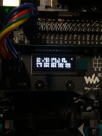
After we follow all the steps and successfully connect the Jetracer to PC, we get a new IP for the Jetracer. Once we get this, we can just dierectly connect to the Jetracer using that. But sometimes the IP changes randomly. So far I have seen '20', '21' and '25' for the last digit. So if there is trouble with the connetion, it is advisable to check the IP which is shown on the small OLED display of Jetracer like the figure below.

Fig. 1: IP on OLED of the Jetracer

Training the Jetracer

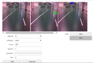
The jetracer is trained using the 'interactive_regression.ipynb' file, which is available inside /jetracer/notebooks. We just need to open the file inside JupyterLab and run all cells. The last program will display the following interface like Figure 2.

Fig. 2: Camera Interface

Inside the interface, the left most window shows the live preview of the camera and this is where we show the car the ideal path by clicking on a point on the track where we would like it to go. Once we click, a photo is taken and saved inside the dataset. The window in the middle shows the photo and the green dot represents the ideal point that we chose. The right most window also shows a live preview, with the blue dot which shows the ideal point on the track where we would like it to follow. In figure 2, the blue dot is not at the ideal path since it had not been trained yet.