Image Processing with MATLAB and AI

| Autor: | Ajay Paul |
| Art: | bachelor thesis |
| Starttermin: | TBD |
| Abgabetermin: | TBD |
| Betreuer: | Prof. Dr.-Ing. Schneider |
| Zweitprüfer: | Mirek Göbel |
Introduction
Signal processing has long been a basis in the analysis and manipulation of data in various domains such as telecommunications, radar, audio processing, and imaging. Signal processing has traditionally focused on analyzing, filtering, and interpreting signals in both the time and frequency domains. With the integration of AI, especially deep learning, the possibilities expand to include noise reduction and more. It is essential in many modern applications such as communications, audio and image processing, biomedical signal analysis, and control systems.
Task list
- Solve the Image Processing Tasks with classic algorithms.
- Research on AI Solutions.
- Evaluation of the solutions using a morphological box (Zwicky box)
- Solve the Image Processing Tasks with AI algorithms.
- Compare the different approaches according to scientific criteria
- Scientific documentation
Getting startes
- You are invited to the image processing class in MATLAB Grader.
- Choose the examples from the categories in table 1. Start with 1 end with 6.
- Solve the tasks with classic algorithms.
- Solve the tasks with AI.
- Save your results in SVN.
- Use MATLAB R2025b for the algorithms.
Image Processing Tasks with classic algorithms
Image Processing: Recovery and restoration of information
| # | Categorie | Grader Lecture |
|---|---|---|
| 1 | Recovery and restoration of information | 5 |
| 2 | Image enhancement | 6 |
| 3 | Noise Reduction | 7 |
| 4 | Data based segmentation | 8 |
| 5 | Model based segmentation | 9 |
| 6 | Classification | 10 |
SVN Repository:
https://svn.hshl.de/svn/MATLAB_Vorkurs/trunk/Signalverarbeitung_mit_Kuenstlicher_Intelligenz
Requirements regarding the Scientific Methodology
- Scientific methodology (project plan, etc.), helpful article: Gantt Diagramm erstellen
- Weekly progress reports (informative), update the Meeting Minutes
- Project presentation in the wiki
- Daily backup of work results in SVN
- Student Projects with Prof. Schneider
- Anforderungen an eine wissenschaftlich Arbeit
→ zurück zum Hauptartikel: Requirements for a scientific project
Convolutional Neural Network for Image Classification
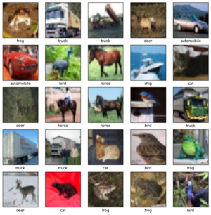
A Convolutional Neural Network (CNN) is a class of deep neural networks, most commonly applied to analyzing visual imagery. This article describes a specific implementation of a CNN using the TensorFlow and Keras libraries to classify images from the CIFAR-10 dataset.
Overview
The model described herein is designed to classify low-resolution color images ($32 \times 32$ pixels) into one of ten distinct classes (e.g., airplanes, automobiles, birds, cats). The implementation utilizes a sequential architecture consisting of a convolutional base for feature extraction followed by a dense network for classification.
Dataset
The system is trained on the CIFAR-10 dataset, which consists of 60,000 $32 \times 32$ color images in 10 classes, with 6,000 images per class.
- Training set: 50,000 images
- Test set: 10,000 images
- Preprocessing: Pixel values are normalized to the range [0, 1] by dividing by 255.0 to accelerate convergence during gradient descent.

Network Architecture
The architecture follows a sequential pattern: Conv2D $\rightarrow$ MaxPooling $\rightarrow$ Dense. The specific layer configuration and parameter counts are detailed below:
Model: "sequential"
| Layer (type) | Output Shape | Param # |
|---|---|---|
| conv2d (Conv2D) | (None, 30, 30, 32) | 896 |
| max_pooling2d (MaxPooling2D) | (None, 15, 15, 32) | 0 |
| conv2d_1 (Conv2D) | (None, 13, 13, 64) | 18,496 |
| max_pooling2d_1 (MaxPooling2D) | (None, 6, 6, 64) | 0 |
| conv2d_2 (Conv2D) | (None, 4, 4, 64) | 36,928 |
| flatten (Flatten) | (None, 1024) | 0 |
| dense (Dense) | (None, 64) | 65,600 |
| dense_1 (Dense) | (None, 10) | 650 |
| Total params: 122,570 (478.79 KB) | ||
| Trainable params: 122,570 (478.79 KB) | ||
| Non-trainable params: 0 (0.00 B) | ||
Implementation Details
Training Configuration
The model is compiled with the following hyperparameters:
- Optimizer: Adam (Adaptive Moment Estimation).
- Loss Function: Sparse Categorical Crossentropy (from_logits=True).
- Metrics: Accuracy.
- Epochs: 10 iterations over the entire dataset.
Performance
Upon training for 10 epochs, the model typically achieves:
- Training Accuracy: High (variable based on initialization).
- Test Accuracy: Approximately 70% – 75%.
- Overfitting: A divergence between training accuracy and validation accuracy suggests the model may memorize training data. Techniques such as Dropout or Data Augmentation are recommended to mitigate this.
Inference on Custom Images
To test the model on high-quality external images, the input must be resized to match the network's input constraints ($32 \times 32$ pixels).
img = image.load_img(path, target_size=(32, 32))
img_array = image.img_to_array(img) / 255.0
predictions = model.predict(img_array)