Image Processing: Image enhancement

Image Enhancement: Histogram Processing

Image Enhancement is the process of adjusting digital images so that the results are more suitable for display or further image analysis. Unlike Image Restoration, which models degradation to recover the "truth," enhancement is subjective and aims to improve the visual perception of information, such as contrast or brightness.

This article focuses on contrast enhancement using specific MATLAB algorithms: Global Histogram Equalization and CLAHE (Contrast Limited Adaptive Histogram Equalization).

Theoretical Background

The Image Histogram

A histogram represents the distribution of pixel intensities in an image. For an 8-bit grayscale image, the x-axis represents the gray levels (0-255) and the y-axis represents the count of pixels at that specific intensity.

• A Low Contrast image has a histogram clustered in a narrow area (e.g., all pixels are mid-gray).
• A High Contrast image has a histogram stretched across the entire dynamic range.

Method A: Global Histogram Equalization (HE)

This algorithm transforms the intensity values of the image so that the histogram of the output image approximately matches a specified distribution (usually uniform).

• Concept: It creates a transformation function based on the Cumulative Distribution Function (CDF).
• Pros: Simple and effective for background separation.
• Cons: Because it uses global statistics, it can "wash out" details or amplify noise in areas that are relatively flat.

Method B: CLAHE

Contrast Limited Adaptive Histogram Equalization operates on small regions in the image, called tiles.

• Adaptive: Each tile's contrast is enhanced, so that the histogram of the output region approximately matches a specified distribution.
• Contrast Limited: To prevent amplifying noise (which is the main drawback of standard Adaptive Histogram Equalization), the contrast enhancement is limited. Neighboring tiles are then combined using bilinear interpolation to remove artificially induced boundaries.

MATLAB Implementation

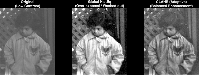
The following script demonstrates the comparison between the original image, Global Histogram Equalization, and CLAHE using the standard MATLAB Image Processing Toolbox.

Code Example

%% Image Enhancement
clc; clear; close all;

% 1. Load a low-contrast image
% 'pout.tif' is a built-in MATLAB demo image suitable for this task
I = imread('pout.tif');

% 2. Method A: Global Histogram Equalization
% This stretches the intensity across the entire 0-255 range based on global stats
I_global = histeq(I);

% 3. Method B: CLAHE (Adaptive Equalization)
% We set a ClipLimit to prevent noise amplification in flat areas
I_clahe = adapthisteq(I, 'ClipLimit', 0.02, 'Distribution', 'rayleigh');

% 4. Visualization
figure('Name', 'Task 2: Image Enhancement Comparison', ...
       'NumberTitle', 'off', ...
       'Position', [100, 100, 1200, 500]);

% Plot Original
subplot(1, 3, 1);
imshow(I);
title({'Original', '(Low Contrast)'}, 'FontSize', 12);

% Plot Global HE
subplot(1, 3, 2);
imshow(I_global);
title({'Global HistEq', '(Over-exposed / Washed out)'}, 'FontSize', 12);

% Plot CLAHE
subplot(1, 3, 3);
imshow(I_clahe);
title({'CLAHE (Adaptive)', '(Balanced Enhancement)'}, 'FontSize', 12, 'FontWeight', 'bold');

% 5. Optional: View Histograms to see the math
% A flat histogram means "perfect" contrast (high entropy).
figure('Name', 'Task 2: Histogram Analysis', 'Position', [100, 100, 1200, 400]);
subplot(1,3,1); imhist(I); title('Original Histogram');
subplot(1,3,2); imhist(I_global); title('Global HE Histogram');
subplot(1,3,3); imhist(I_clahe); title('CLAHE Histogram');

Detailed Code Logic

1. Data Loading

I = imread('pout.tif');

We use pout.tif because it is a classic example of a low-contrast grayscale image (the histogram is bunched in the center). If working with color images, one must convert to grayscale (rgb2gray) or convert to the Lab color space and applying enhancement only to the 'L' (Luminance) channel to avoid distorting colors.

2. Global Equalization (Method A)

I_global = histeq(I);

The function histeq computes the CDF of the image. It generates a transformation $T(r)$ where $r$ is the input intensity. It maps input pixels to output pixels such that the output histogram is flat (uniform).

• Observation: In the result, the background of the image often becomes too bright or noisy because the algorithm blindly forces the statistics to cover the whole range.

3. Adaptive Equalization (Method B)

I_clahe = adapthisteq(I, 'ClipLimit', 0.02, 'Distribution', 'rayleigh');

The function adapthisteq is more sophisticated:

• ClipLimit (0.02): This parameter controls the contrast limit. A higher number yields more contrast but also more noise. 0.01 to 0.03 is the standard range.
• Distribution ('rayleigh'): Instead of a uniform distribution, we use 'rayleigh' (bell-curve shaped), which produces a more natural look than the harsh flat line of uniform distribution.

4. Visualization

The code uses subplot(1,3,x) to display images side-by-side.

• Original: Looks gray and dull.
• Global HE: Looks harsh; the girl's face might be overly bright (washed out).
• CLAHE: Looks natural; details in the coat and face are visible without saturation.

Comparison of Techniques

Feature	Global Histogram Equalization (HE)	CLAHE
Scope	Uses pixels from the entire image	Uses local tiles (e.g., 8x8 blocks)
Contrast	Maximum possible (often excessive)	Controlled (user-defined limit)
Noise	Amplifies background noise significantly	Limits noise amplification via clipping
Use Case	Scientific imaging (thermal, X-ray) where raw data separation is key	Photography, medical imaging (MRI/CT), underwater vision
MATLAB Function	histeq()	adapthisteq()