Image Processing: Noise Reduction

Noise Reduction: Median vs. Linear Filtering

Noise Reduction is a fundamental step in image processing used to improve image quality by removing unwanted signal artifacts (noise) while preserving important structural features like edges and textures.

This article explores the specific problem of removing Salt & Pepper Noise (Impulse Noise) and demonstrates why non-linear filtering (Median) is superior to linear filtering (Averaging) for this specific type of degradation.

Theoretical Background

Salt & Pepper Noise

Salt & Pepper noise presents itself as sparsely occurring white and black pixels. It typically arises from:

• Errors in data transmission.
• Malfunctioning pixel elements in camera sensors.
• Analog-to-digital converter errors.

In an 8-bit image, "Salt" is a pixel value of 255 (white) and "Pepper" is a pixel value of 0 (black). Unlike Gaussian noise, which modifies values by small amounts, Salt & Pepper noise replaces the original pixel value entirely with an extrema value.

The Solution: Median Filtering

The Median Filter is a non-linear digital filtering technique.

1. It looks at a neighborhood of pixels (e.g., a 3x3 square) around a target pixel.
2. It sorts all pixel values in that neighborhood in numerical order.
3. It replaces the target pixel with the median (middle) value of the sorted list.

Why it works: The median is robust against outliers. Since Salt & Pepper pixels are mathematical outliers (0 or 255), they usually end up at the very start or very end of the sorted list, ensuring the median value picked is a "real" neighbor pixel.

The Comparison: Linear Average Filtering

A Linear Average (Mean) Filter calculates the arithmetic mean of the neighborhood and replaces the center pixel with that mean.

• The Problem: If a 3x3 neighborhood contains just one "Salt" pixel (255) on a black background (0), the average will be $(255+0+...)/9\approx 28$.
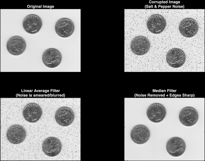
• Result: The bright white dot becomes a gray smudge. The noise is spread out (blurred) rather than removed.

MATLAB Implementation

The following MATLAB script demonstrates the creation of noise, the application of both filters, and the visual comparison.

Code Logic

% Noise Reduction
% Algorithm: Median Filtering (medfilt2)
clc; clear; close all;

% 1. Load a clean image
% 'eight.tif' is a standard high-contrast binary-style image provided in MATLAB
I = imread('eight.tif');

% 2. Add Salt & Pepper Noise
% Density 0.05 means approximately 5% of the pixels are corrupted.
noise_density = 0.05;
I_noisy = imnoise(I, 'salt & pepper', noise_density);

% 3. Apply Median Filter (The Classic Algorithm)
% 'medfilt2' performs 2-D median filtering. [3 3] is the window size.
I_median = medfilt2(I_noisy, [3 3]);

% 4. Comparison: Linear Average Filter
% We create a 3x3 averaging kernel (box filter)
h = fspecial('average', [3 3]);
% Apply the linear filter
I_average = imfilter(I_noisy, h);

% 5. Visualization
figure('Name', 'Task 3: Noise Reduction', 'Position', [100, 100, 1200, 800]);

% A. Original
subplot(2, 2, 1); imshow(I);
title('Original Image', 'FontSize', 12);

% B. Noisy
subplot(2, 2, 2); imshow(I_noisy);
title({'Corrupted Image', '(Salt & Pepper Noise)'}, 'FontSize', 12);

% C. Average Filter Result
subplot(2, 2, 3); imshow(I_average);
title({'Linear Average Filter', '(Noise is smeared/blurred)'}, 'FontSize', 12);

% D. Median Filter Result
subplot(2, 2, 4); imshow(I_median);
title({'Median Filter', '(Noise Removed + Edges Sharp)'}, 'FontSize', 12, 'FontWeight', 'bold');

Analysis of Results

Visual Comparison

Filter Type	Effect on Noise	Effect on Edges	Conclusion
Average Filter	Reduces the intensity of the noise dots but spreads them out, creating "blobs" or smudges.	Edges become blurred. The image loses sharpness.	Incorrect method for Impulse noise.
Median Filter	Completely removes the white and black dots (assuming noise density isn't too high).	Edges remain sharp because no averaging takes place across the edge boundary.	Correct method for Impulse noise.

Parameter Sensitivity

• Window Size ([3 3]): A 3x3 window works well for low noise densities (like 0.05). If the noise density increases (e.g., > 0.2), a larger window (5x5) might be required to ensure the median value isn't a noise pixel itself, though this will result in loss of fine detail.

Key MATLAB Functions

• imnoise(I, 'salt & pepper', D): Adds impulse noise with density $D$.
• medfilt2(I, [m n]): Performs 2D median filtering using an $m\times n$ window.
• fspecial('average', [m n]): Creates a linear averaging filter kernel.
• imfilter(I, h): Convolves the image $I$ with kernel $h$.